Wind engineering

Wind and structural health monitoring is an essential step of the validation of the buffeting theory, which describes the wind-induced response of a structure to atmospheric turbulence. The Lysefjord suspension Bridge has been used since 2013 as a full-scale wind engineering laboratory and is currently instrumented with eleven 3D sonic anemometers, three pressure probes, four pairs of tri-axial accelerometers inside the deck deck and a GNNS based displacement sensor. This makes the bridge one of the world's most densely instrumented suspension bridge in terms of wind sensors. A master data logging unit synchronizes the data into a single data file, which is then continuously transmitted via mobile net. The recently introduced pressure signals are stored and transmitted separately.

Go back

The deployment of Structural Health Monitoring systems (SHMS) on long-span suspension bridges aims to identify the modal parameters of such structures, i.e. its eigenfrequencies, mode shapes and damping ratios. Accelerometers are traditionally used to monitor the dynamic response, but Global Navigation Satellite Systems (GNSS) have been increasingly used for the last 20 years for a similar purpose. SHMS introduces also a possibility to study the influence of the temperature on the bridge dynamic characteristics. Wind and Structural Health Monitoring systems (WASHMS) include wind velocity measurements from the bridge deck. Although WASHMS are uncommon, they allow a direct study of the wind-induced vibrations of the bridge.

The Lysefjord bridge is a suspension bridge with a main span of 446 m, crossing the inlet of a narrow and long fjord (Fig. 1). The fjord is enclosed by mountains and steep hills that channel the flow, such that two main wind directions are primarily observed. The first sector corresponds to a flow from north-northeast, i.e. from the inside of the fjord, at azimuth between 0° and 60°. The second one corresponds to a flow from south-southwest, i.e. a wind direction between 180° and 270°. The Lysefjord bridge has been instrumented with a wind and structural health monitoring system since November 2013. In June 2017, the arrangement of the wind sensors was modified and three sonic anemometers were installed on the east side of the bridge. In July 2020, two sonic anemometers were installed upstream and downstream of the bridge deck, at the deck level, as part of a study of bridge deck aerodynamics in full-scale.

In Fig. 2, the position of the anemometers above the deck is defined using the hanger name HXY, where X is a digit between 08 and 24 indicating the hanger number, and Y denotes the west side (W) or east side (E) of the deck. Since two anemometers are mounted on the west hanger no. 08 (H08W), the notations H08Wb and H08Wt refer to the sonic anemometer mounted 6 m (bottom) and 10 m (top) above the deck, respectively. The two anemometers at the bridge deck level are designated D08W and D08W.

The accelerometers used are triaxial MEMs (microelectromechanical systems) silicon accelerometers from Canterbury Seismic Instruments Ltd. Figure 3 shows an accelerometer within the bridge deck. Each section of the bridge has two sensors, one on either side of the bridge deck, to monitor the bridge twisting response in addition to the translational responses. The lateral distance between two accelerometers constituting a pair is ca. 7.15 m and the maximal sampling frequency of each accelerometer is 200 Hz.

In addition, the displacement of the bridge deck is monitored using a Real-Time Kinematic-Global Positioning System (RTK-GPS). More precisely, as the rover is located on top of the main cable, it is the displacement of the main cable in the middle of the bridge span, approximatively 3 m above the bridge girder that is being observed. The RTK-GPS base-rover combination improves the accuracy of measurements by recording the relative displacement between a "fixed" base station on the northwest side and a "moving" rover station located on the main cable at mid-span. Naturally, the accuracy varies depending on the quality of the instruments used. In the present case, a set of Trimble BD930 GNSS receivers are coupled to Trimble AV33 GNSS antennas. These sensors can handle data sampling at a frequency of 20 Hz, with an accuracy of \( \pm 8 \) mm \(+ 1 \) ppm for the horizontal displacements and \( \pm 15 \) mm \(+1 \) ppm for the vertical displacements. The GPS technique is ideal for tracking the performances of long-span suspension bridges due to their low natural frequency and large amplitude displacements.

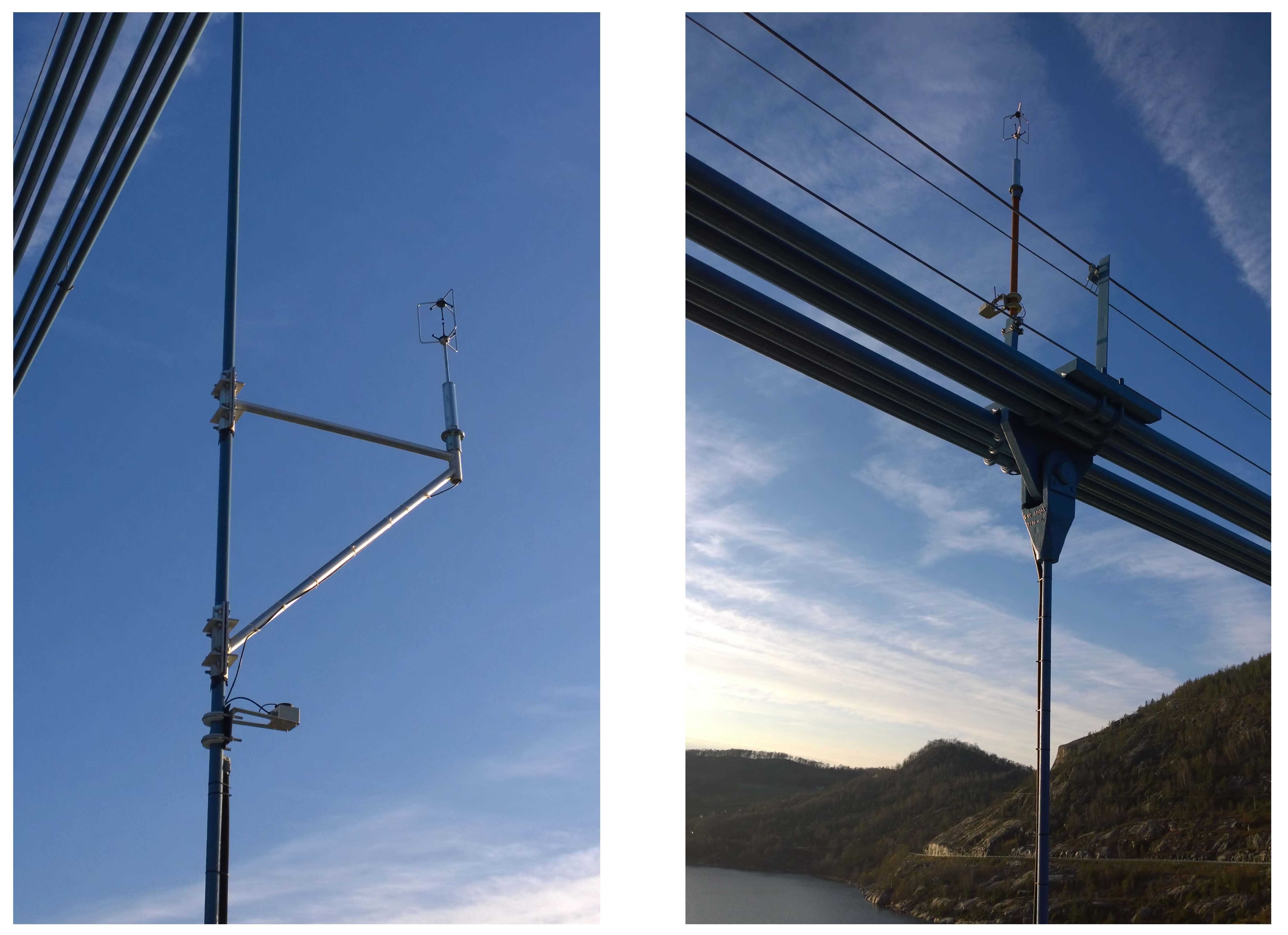
Eight of the sonic anemometers are 3-D WindMaster Pro from Gill instruments (Lymington, UK), which can operate with a sampling frequency up to 32 Hz. A 2-D sonic anemometer, mounted on H10W, is a Weather Transmitter WXT520 from Vaisala (Helsinki, Finland), which monitors the horizontal wind components, rainfall, relative humidity, pressure and absolute temperature with a sampling frequency up to 4 Hz. The anemometers are either mounted directly on brackets that are fixed to the hangers (Fig. 5, left), or placed on the top of a 2.5-m long vertical steel pole placed above the main cables and fixed to the safety railings for the main cables (Fig. 5, right). Two additional 3-D anemometers supported by a horizontal pole (3-D WindMaster HS) are fixed to a bracket anchored to the bridge deck railing.

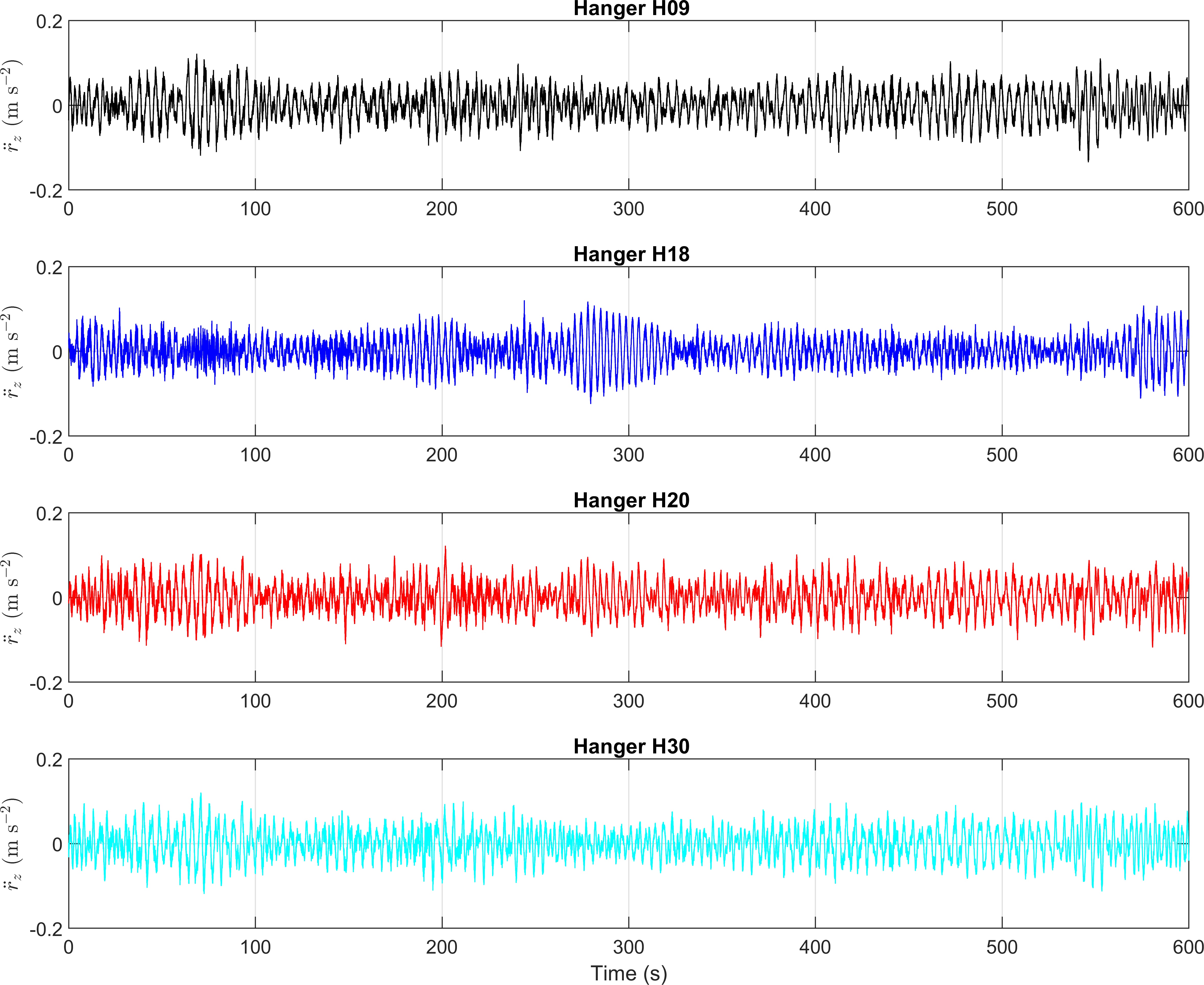
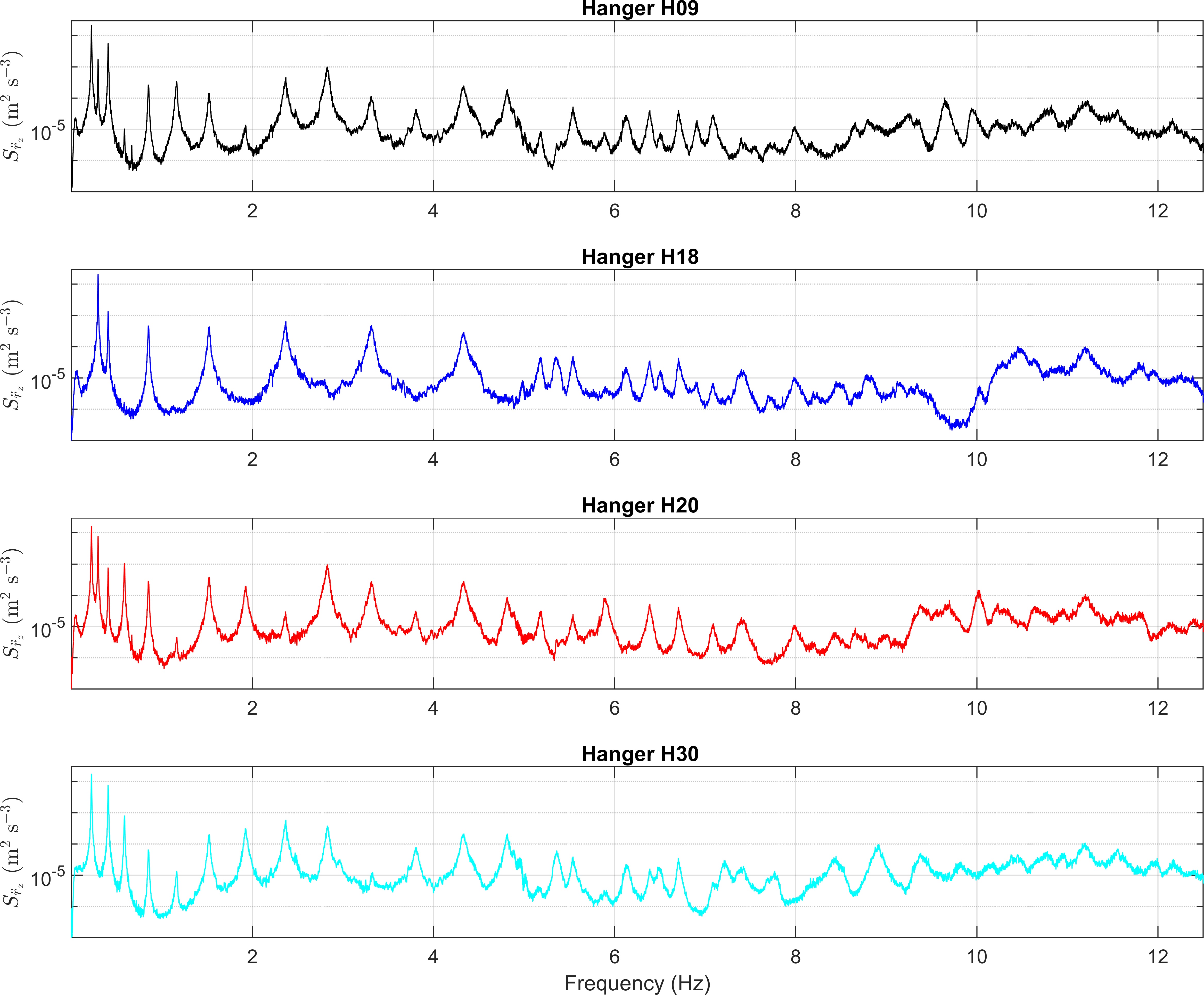
Figure 6 shows ten minutes of lateral acceleration data recorded by the four pairs of accelerometers near hangers 09, 18, 20 and 30. These records correspond to wind-induced vibrations rather than traffic-induced vibrations. At midspan (H18), the bridge response is dominated by a single mode of vibration with a period of ca. 7.4 s. In the frequency domain, the associated power spectral density estimates of the lateral bridge acceleration response are displayed in Fig. 7. The different peaks correspond to the lateral eigen-frequencies of the bridge.

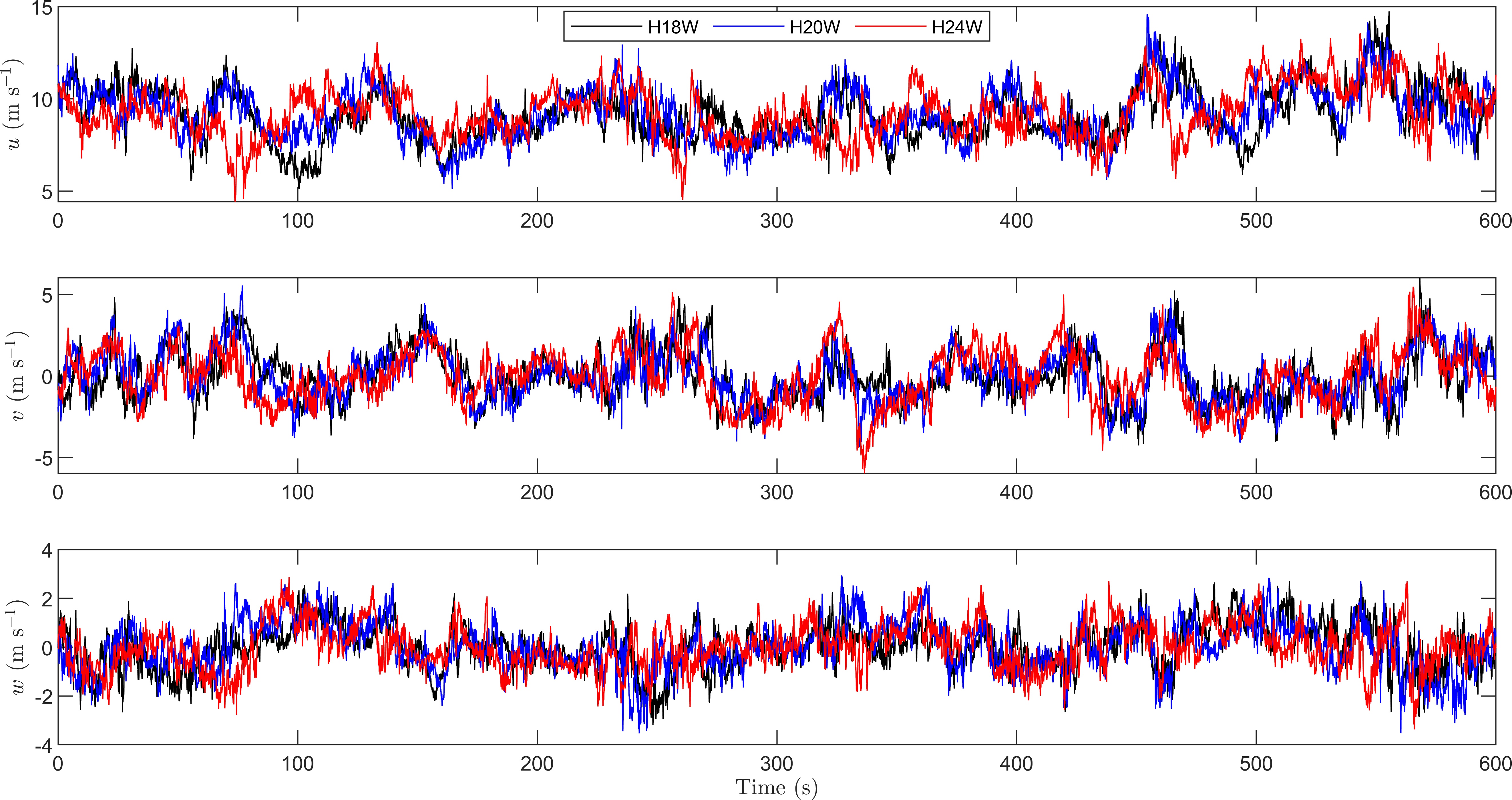
Figure 8 shows ten minutes of velocity data recorded by three of the sonic anemometers on the west side of the bridge deck, for a flow from south-southwest. The top panel shows the \(u\) component, the middle one the \(v\) component and the bottom panel corresponds to the \(w\) component. For a given wind component, the time series are clearly correlated between each other, which reflects the existence of coherent structures.

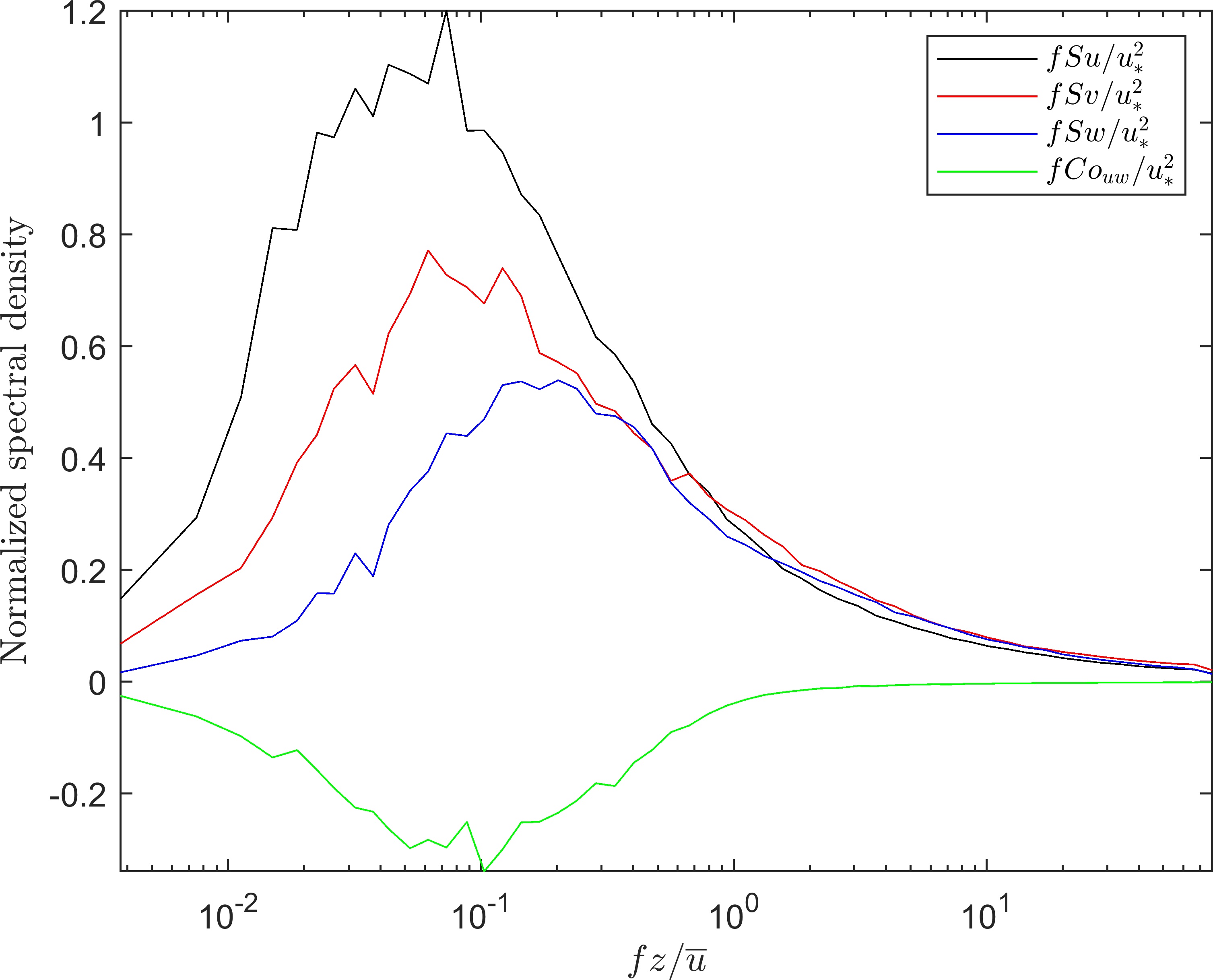
Figure 9 shows the single-point auto and cross-power spectral densities for each of the component recorded on the east side of the bridge, for a flow from north-northeast. The sonic anemometer used here is the one on H18E. The data set considered corresponds to several months of measurements, from July 2017 to June 2018, but only the samples associated with a wind direction between 0° and 60° at midspan have been selected.